The ggchemplot R package

The workflow of ggchemplot follows three steps:

1. Parse a SDF file with ggchemplot1().
   
2. Visualize the preliminary plot and modify the data with helper functions for polishing.
   
3. Plot the final visualization with ggchemplot2().

Short tutorial

Install the package from my GitHub repository.

# Install the remotes package if not already installed
install.packages("remotes")

# Install ggchemplot from GitHub
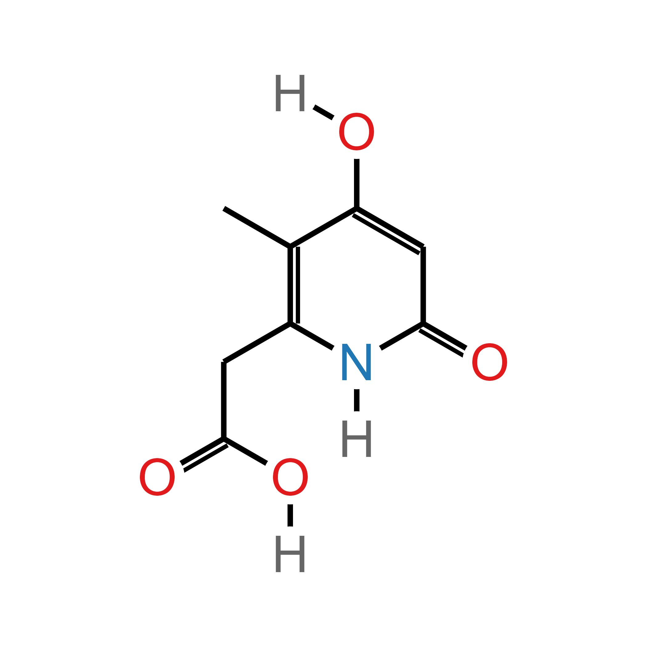
remotes::install_github("JPFQueiroz/ggchemplot")

The input file in this example (P1_pyridone.sdf) was prepared through the drawing tool of PubChem. Other R users might also prepare the input structure directly from R with rcdk (Guha, 2007). Use ggchemplot1 to parse the file and generate the initial data object.

# Load ggchemplot
library(ggchemplot)

# Parse the data and generate initial plot
p1 <- ggchemplot1(sdf_file = "P1_pyridone.sdf")

# Check the initial plot
p1$plot

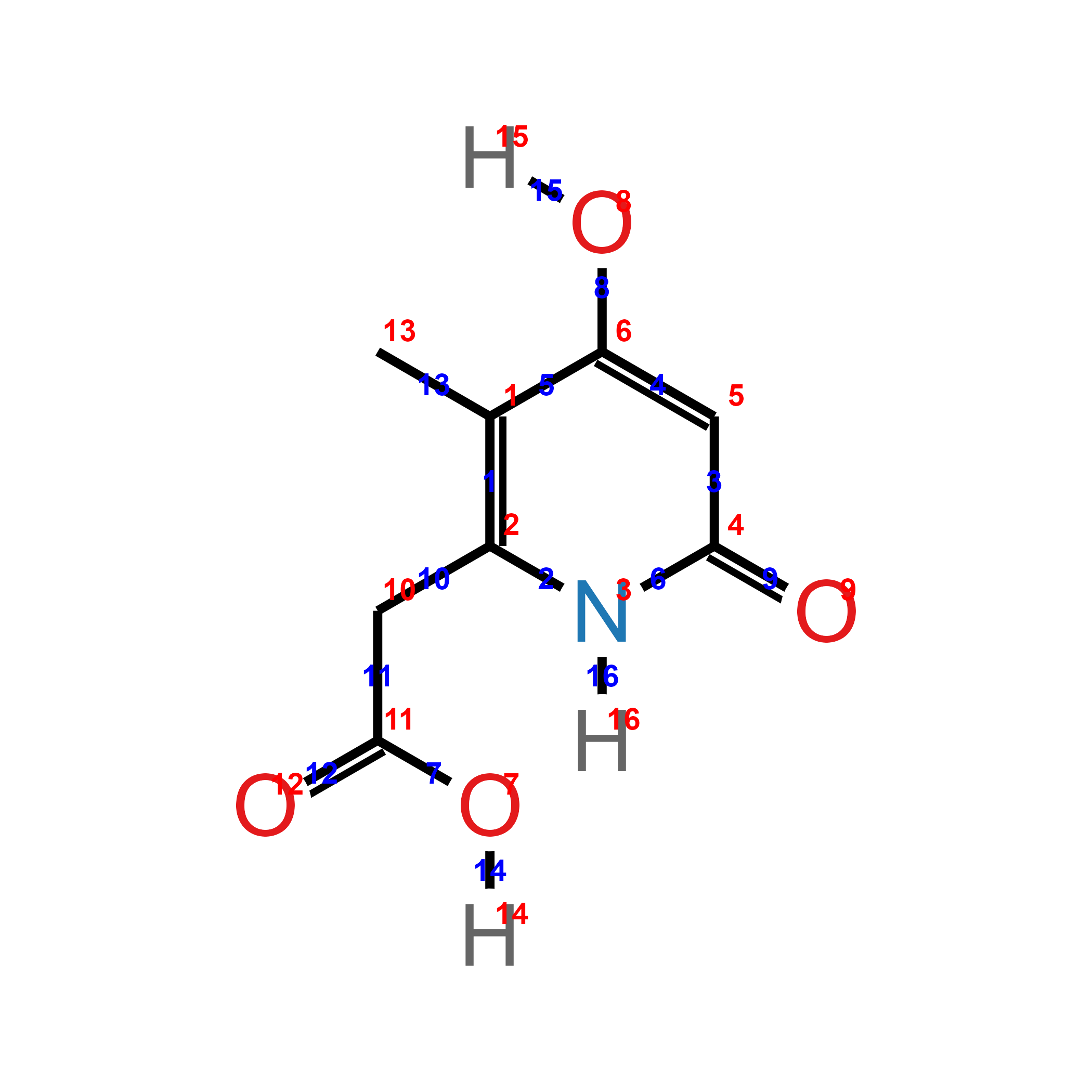
Quickly visualize the atom and bond ids in p1$atoms on the plot with the argument show_ids = TRUE in ggchemplot2(). The ids visualization can guide through the polishing step, where many functions use as argument ids of atoms or bonds.

# Load dplyr to use the pipe operator %>% 
library(dplyr)

p1 %>% 
  ggchemplot2(show_ids = TRUE)

Polish the visualization using the arguments available in ggchemplot1(), modifying the underlying data with helper functions or through manual wrangling of the dataframe objects, and finally to ggchemplot2().

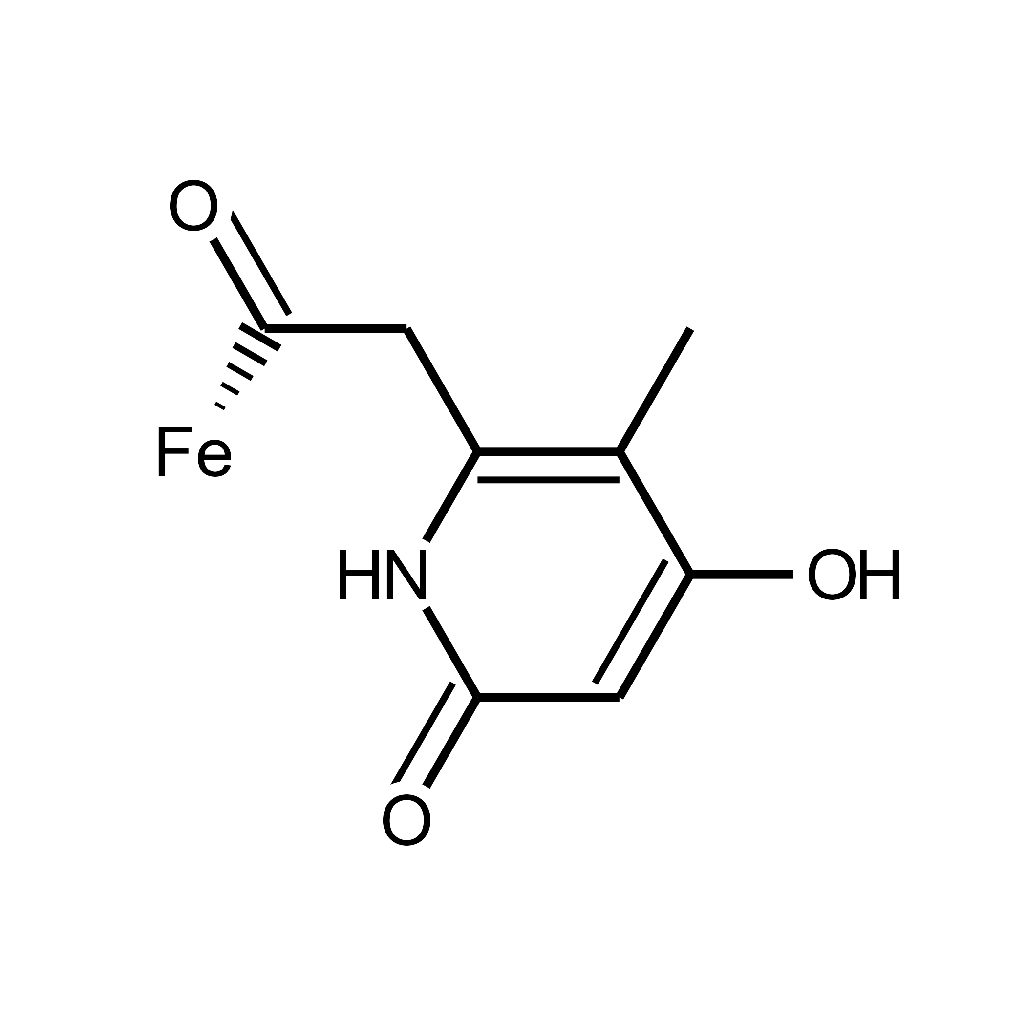
# Publication-quality plot
p1 <- ggchemplot1(
  sdf_file = "P1_pyridone.sdf",
  title = NULL,
  collapse_hydrogens = TRUE,
  rotation = 90,
  label_padding = 1,
  show_atom_circles = TRUE,
  hide_carbon_circles = TRUE,
  circle_stroke = 0,
  show_atom_labels = TRUE,
  hide_carbon_labels = TRUE,
  bond_width = 2,
  atom_size = 18,
  label_size = 12,
  double_bond_offset = 0.3,
  custom_atom_colors = NULL,
  paint_it_black = TRUE,
  H_offset = c(0.50, 1)) %>% 
  change_label(atom_id = 7, new_label = "Fe") %>% 
  add_hashed_bond(from_id = 7, to_id = 11, 
                  wedge_thickness = 0.3,n_hashes = 6,
                  shorten = c(0.3, 0)) %>% 
  ggchemplot2()

# Plot
p1

The basic tutorial ends here. You can cite ggchemplot (Fernandes-Queiroz, 2026) in your publications using the BibTex citation below. Your feedback is welcome.

@software{ggchemplot,
  author       = {João Pedro Fernandes Queiroz},
  title        = {JPFQueiroz/ggchemplot: ggchemplot: an R package for visualization of chemical structures},
  month        = may,
  year         = 2026,
  publisher    = {Zenodo},
  version      = {v0.2-beta.1},
  doi          = {10.5281/zenodo.20088880},
  url          = {https://doi.org/10.5281/zenodo.20088880},
}